eifueo/docs/1a/math117.md

MATH 117: Calculus 1

Functions

A function is a rule where each input has exactly one output, which can be determined by the vertical line test.

!!! definition - The domain is the set of allowable independent values. - The range is the set of allowable dependent values.

Functions can be composed to apply the result of one function to another. $(f\circ g)(x) = f(g(x))$

!!! warning Composition is not commutative: $f\circ g \neq g\circ f$.

Inverse functions

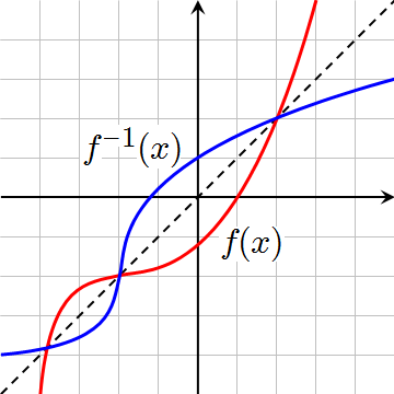
The inverse of a function swaps the domain and range of the original function: $f^{-1}(x)$ is the inverse of $f(x)$.. It can be determined by solving for the other variable: \[ \begin{align*} y&=mx+b \\ y-b&=mx \\ x&=\frac{y-b}{m} \end{align*} \]

Because the domain and range are simply swapped, the inverse function is just the original function reflected across the line $y=x$.

(Source: Wikimedia Commons, public domain)

If the inverse of a function is applied to the original function, the original value is returned. $f^{-1}(f(x)) = x$

A function is invertible only if it is “one-to-one”: each output must have exactly one input. This can be tested via a horizontal line test of the original function.

If a function is not invertible, restricting the domain may allow a partial inverse to be defined.

!!! example (Source: Wikimedia Commons, public domain) By restricting the domain to $[0,\inf]$, the multivalued inverse function $y=\pm\sqrt{x}$ is reduced to just the partial inverse $y=\sqrt{x}$.

Symmetry

An even function satisfies the property that $f(x)=f(-x)$, indicating that it is unchanged by a reflection across the y-axis.

An odd function satisfies the property that $-f(x)=f(-x)$, indicating that it is unchanged by a 180° rotation about the origin.

The following properties are always true for even and odd functions:

• even × even = even
• odd × odd = even
• even × odd = odd

Functions that are symmetric (that is, both $f(x)$ and $f(-x)$ exist) can be split into an even and odd component. Where $g(x)$ is the even component and $h(x)$ is the odd component: \[ \begin{align*} f(x) &= g(x) + h(x) \\ g(x) &= \frac{1}{2}(f(x) + f(-x)) \\ h(x) &= \frac{1}{2}(f(x) - f(-x)) \end{align*} \]

!!! note The hyperbolic sine and cosine are the even and odd components of $f(x)=e^x$. $\cosh x = \frac{1}{2}(e^x + e^{-x}) \\ \sinh x = \frac{1}{2}(e^x - e^{-x})$

Piecewise functions

A piecewise function is one that changes formulae at certain intervals. To solve piecewise functions, each of one’s intervals should be considered.

Absolute value function

\[ \begin{align*} |x| = \begin{cases} x &\text{ if } x\geq 0 \\ -x &\text{ if } x < 0 \end{cases} \end{align*} \]

Signum function

The signum function returns the sign of its argument.

\[ \begin{align*} \text{sgn}(x)=\begin{cases} -1 &\text{ if } x < 0 \\ 0 &\text{ if } x = 0 \\ 1 &\text{ if } x > 0 \end{cases} \end{align*} \]

Ramp function

The ramp function makes a ramp through the origin that suddenly flatlines at 0. Where $c$ is a constant:

\[ \begin{align*} r(t)=\begin{cases} 0 &\text{ if } x \leq 0 \\ ct &\text{ if } x > 0 \end{cases} \end{align*} \]

(Source: Wikimedia Commons, public domain)

Floor and ceiling functions

The floor function rounds down. $\lfloor x\rfloor$

The ceiling function rounds up. $\lceil x \rceil$

Fractional part function

In a nutshell, the fractional part function:

• returns the part after the decimal point if the number is positive
• returns 1 - the part after the decimal point if the number is negative

$\text{FRACPT}(x) = x-\lfloor x\rfloor$

Because this function is periodic, it can be used to limit angles to the $[0, 2\pi)$ range with: $f(\theta) = 2\pi\cdot\text{FRACPT}\biggr(\frac{\theta}{2\pi}\biggr)$

Heaviside function

The Heaviside function effectively returns a boolean whether the number is greater than 0. \[ \begin{align*} H(x) = \begin{cases} 0 &\text{ if } t < 0 \\ 1 &\text{ if } t \geq 0 \end{cases} \end{align*} \]

This can be used to construct other piecewise functions by enabling them with $H(x-a)$ as a factor, where $a$ is the interval.

In a nutshell:

• $1-H(t-a)$ lets you “turn a function off” at at $t=a$
• $H(t-a)$ lets you “turn a function on at $t=a$
• $H(t-a) - H(t-b)$ leaves a function on in the interval $(a, b)$

!!! example TODO: example for converting piecewise to heaviside via collecting heavisides

and vice versa

Periodicity

The function $f(t)$ is periodic only if there is a repeating pattern, i.e. such that for every $x$, there is an $f(x) = f(x + nT)$, where $T$ is the period and $n$ is any integer.

Circular motion

Please see SL Physics 1#6.1 - Circular motion and its subcategory “Angular thingies” for more information.

Partial function decomposition (PFD)

In order to PFD:

1. Factor the denominator into irreducibly quadratic or linear terms.
2. For each factor, create a term. Where capital letters below are constants:

• A linear factor $Bx+C$ has a term $\frac{A}{Bx+C}$.
• An irreducibly quadratic factor $Dx^2+Ex+G$ has a term $\frac{Hx+J}{Dx^2+Ex+G}$.
• Duplicate factors have terms with denominators with that factor to the power of 1 up to the number of times the factor is present in the original.

4. Set the two equal to each other such that the denominators can be factored out.
5. Create systems of equations to solve for each constant.

!!! example To decompose $\frac{x}{(x+1)(x^2+x+1)}$: \[ \begin{align*} \frac{x}{(x+1)(x^2+x+1)} &= \frac{A}{x+1} + \frac{Bx+C}{x^2+x+1} \\ &= \frac{A(x^2+x+1) + (Bx+C)(x+1)}{(x+1)(x^2+x+1)} \\ x &= A(x^2+x+1) + (Bx+C)(x+1) \\ 0x^2 + x + 0 &= (Ax^2 + Bx^2) + (Ax + Bx + Cx) + (A + C) \\ \\ &\begin{cases} 0 = A + B \\ 1 = A + B + C \\ 0 = A + C \end{cases} \\ A &= -1 \\ B &= 1 \\ C &= 1 \\ \\ ∴ \frac{x}{(x+1)(x^2+x+1)} &= -\frac{1}{x+1} + \frac{x + 1}{x^2 + x + 1} \end{align*} \]

Trigonometry

1 radian represents the angle when the length of the arc of a circle is equal to the radius. Where $s$ is the arc length:

$\theta=\frac{s}{r}$

The following table indicates the special angles that should be memorised:

Angle (rad)	0	$\frac{\pi}{6}$	$\frac{\pi}{4}$	$\frac{\pi}{3}$	$\frac{\pi}{2}$	$\pi$
cos	1	$\frac{\sqrt{3}}{2}$	$\frac{\sqrt{2}}{2}$	$\frac{1}{2}$	0	-1
sin	0	$\frac{1}{2}$	$\frac{\sqrt{2}}{2}$	$\frac{\sqrt{3}}{2}$	1	0
tan	0	$\frac{\sqrt{3}}{3}$	1	$\sqrt{3}$	not allowed	0

Identities

The Pythagorean identity is the one behind right angle triangles:

$\cos^2\theta+\sin^2\theta = 1$

Cosine and sine can be converted between by an angle shift:

$\cos\biggr(\theta-\frac{\pi}{2}\biggr) = \sin\theta \\ \sin\biggr(\theta-\frac{\pi}{2}\biggr) = \cos\theta$

The angle sum identities allow expanding out angles:

$\cos(a+b)=\cos a\cos b - \sin a\sin b \\ \sin(a+b)=\sin a\cos b + \cos a\sin b$

Subtracting angles is equal to the conjugates of the angle sum identities.

The double angle identities simplify the angle sum identity for a specific case.

$\sin2\theta = 2\sin\theta\cos\theta \\$

The half angle formulas are just random shit.

$1+\tan^2\theta = \sec^2\theta \\ \cos^2\theta = \frac{1}{2}(1+\cos2\theta) \\ \sin^2\theta = \frac{1}{2}(1-\cos2\theta)$

Inverse trig functions

Because extending the domain does not pass the horizontal line test, for engineering purposes, inverse sine is only the inverse of sine so long as the angle is within $[-\frac{\pi}{2}, \frac{\pi}{2}]$. Otherwise, it is equal to that version mod 2 pi.

$y=\sin^{-1}x \iff x=\sin y, y\in [-\frac{\pi}{2}, \frac{\pi}{2}]$

This means that $x\in[-1, 1]$.

$\sin(\sin^{-1}x) = x \\ \sin^{-1}(\sin x) = x \text{ only if } x\in[-\frac{\pi}{2}, \frac{\pi}{2}]$

Similarly, inverse cosine only returns values within $[0,\pi]$.

Similarly, inverse tangent only returns values within $(-\frac{\pi}{2}, \frac{\pi}{2})$. However, $\tan^{-1}$ is defined for all $x\in\mathbb R$.

Although most of the reciprocal function rules can be derived, secant is only valid in the odd range $[-\pi, -\frac{\pi}{2})\cup [0, \frac{\pi}{2})$, and returns values $(-\infty, -1]\cup [1, \infty)$.

Electrical signals

Waves are commonly presented in the following format, where $A$ is a positive amplitude:

$g(t)=A\sin(\omega t + \alpha)$

In general, if given a sum of a sine and cosine:

$a\sin\omega t + b\cos\omega t = \sqrt{a^2 + b^2}\sin(\omega t + \alpha)$

The sign of $\alpha$ should be determined via its quadrant via the signs of $a$ (sine) and $b$ (cosine) via the CAST rule.

!!! example Given $y=5\cos 2t - 3\sin 2t$:

$$
\begin{align*}
A\sin (2t+\alpha) &= A\sin 2t\cos\alpha + A\cos 2t\sin\alpha \\
&= (A\cos\alpha)\sin 2t + (A\sin\alpha)\cos 2t \\
\\
\begin{cases}
A\sin\alpha = 5 \\
A\cos\alpha = -3
\end{cases}
\\
\\
A^2\sin^2\alpha + A^2\cos^2\alpha &= 5^2 + (-3)^2 \\
A^2 &= 34 \\
A &= \sqrt{34} \\
\\
\alpha &= \tan^{-1}\frac{5}{3} \\
&\text{since sine is positive and cosine is negative, the angle is in Q3} \\
∴ \alpha &= \tan^{-1}\frac{5}{3} + \pi
\end{align*}
$$

Limits

Limits of sequences

!!! definition - A sequence is an infinitely long list of numbers with the domain of all natural numbers (may also include 0). - A sequence that does not converge is a diverging sequence.

A sequence is typically denoted via braces.

$\{a_n\}\text{ or } \{a_n\}^\infty_{n=0}$

Sometimes sequences have formulae.

$\left\{\frac{5^n}{3^n}\right\}^\infty_{n=0}$

The limit of a sequence is the number $L$ that the sequence converges to as $n$ increases, which can be expressed in either of the two ways below:

$a_n \to L \text{ as } n\to\infty \\ \lim_{n\to\infty}a_n=L$

: > Specifically, a sequence $\{a_n\}$ converges to limit $L$ if, for any positive number $\epsilon$, there exists an integer $N$ such that $n>N \Rightarrow |a_n - L | < \epsilon$.

Effectively, if there is always a term number that would lead to the distance between the sequence at that term and the limit to be less than any arbitrarily small $\epsilon$, the sequence has the claimed limit.

!!! example A limit can be proved to exist with the above definition. To prove $\left\{\frac{1}{\sqrt{n}}\right\}\to0$ as $n\to\infty$: \[ \begin{align*} \text{Proof:} \\ n > N &\Rightarrow \left|\frac{1}{\sqrt{n}} - 0\right| < \epsilon \\ &\Rightarrow \frac{1}{\epsilon^2} < n \end{align*} \\ \ce{Let \epsilon\ be any positive number{.} If n > \frac{1}{\epsilon^2}, then \frac{1}{\sqrt{n}}-> 0 as n -> \infty{.}} \]

Please see SL Math - Analysis and Approaches 1#Limits for more information.

The squeeze theorem states that if a sequence lies between two other converging sequences with the same limit, it also converges to this limit. That is, if $a_n\to L$ and $c_n\to L$ as $n\to\infty$, and $a_n\leq b_n\leq c_n$ is always true, $b_n\to L$.

!!! example $\left\{\frac{\sin n}{n}\right\}$: since $-1\leq\sin n\leq 1$, $\frac{-1}{n}\leq\frac{\sin n}{n}\leq \frac{1}{n}$. Since both other functions converge at 0, and sin(n) is always between the two, sin(n) thus also converges at 0 as n approaches infinity.

If function $f$ is continuous and $\lim_{n\to\infty}a_n$ exists:

$\lim_{n\to\infty}f(a_n)=f\left(\lim_{n\to\infty}a_n\right)$

On a side note:

$\lim_{n\to\infty}\tan^{-1} n = \frac{\pi}{2}$

Limits of functions

The definition is largely the same as for the limit of a sequence:

A function $f(x)\to L$ as $x\to a$ if, for any positive $\epsilon$, there exists a number $\delta$ such that $0<|x-a|<\delta\Rightarrow|f(x)-L|<\epsilon$.

Again, for the limit to be true, there must be a value $x$ that makes the distance between the function and the limit less than any arbitrarily small $\epsilon$.

The extra $0 <$ is because the behaviour for when $x=a$, which may or may not be defined, is irrelevant.

!!! example To prove $3x-2\to 4$ as $x\to 2$: \[ \ce{for any \epsilon\ > 0, there is a \delta\ > 0\ such that:} \] \[ \begin{align*} |x-2| < \delta &\Rightarrow|(3x-2) - 4| &< \epsilon \\ &\Leftarrow |(3x-2) -4| &< \epsilon \\ &\Leftarrow |3x-6| &< \epsilon \\ &\Leftarrow |x-2| &< \frac{\epsilon}{3} \\ \delta &= \frac{\epsilon}{3} \end{align*} \] \[ \ce{Let \epsilon\ be any positive number{.} If }|x-2|<\frac{\epsilon}{3}, \\ \text{then }|(3x-2)-4|<\epsilon\text{. Therefore }3x-2\to 4\text{ as }x\to 2. \]

!!! warning When solving for limits, negatives have to be considered if the limit approaches a negative number:

$$\lim_{x\to -\infty}\frac{x}{\sqrt{4x^2-3}} = \frac{1}{-\frac{1}{\sqrt{x}^2}\sqrt{4x^2-3}}$$

As the angle in radians of an arc approaches 0, it is nearly equal to the sine (vertical component).

$\lim_{\theta\to 0}\frac{\sin\theta}{\theta} = 1$

This function is commonly used in engineering and is known as the sinc function.

$\text{sinc}(x) = \begin{cases} \frac{\sin x}{x}&\text{ if }x\neq 0 \\ 0&\text{ if }x=0 \end{cases}$

Continuity

Please see SL Math - Analysis and Approaches 1#Limits and continuity for more information.

Most common functions can be assumed to be continuous (e.g., $\sin x,\cos x, x, \sqrt{x}, \frac{1}{x}, e^x, \ln x$, etc.).

$f(x)$ is continuous in an interval if for any $x$ and $y$ in the interval and any positive number $\epsilon$, there exists a number $\delta$ such that $|x-y|<\delta\Rightarrow |f(x)-f(y)| < \epsilon$.

Effectively, if $f(x)$ can be made infinitely close to $f(y)$ by making $x$ closer to $y$, the function is continuous.

If two functions are continuous:

• $(f\circ g)(x)$ is continuous
• $(f\pm g)(x)$ is continuous
• $(fg)(x)$ is continuous
• $\frac{1}{f(x)}$ is continuous anywhere $f(x)\neq 0$

Intermediate value theorem

The IVT states that if a function is continuous and there is a point between two other points, its term must also be between those two other points.

If $f(x)$ is continuous, if $f(a)\leq C\leq f(b)$, there must be a number $c\in[a,b]$ where $f(c)=C$.

The theorem is used to validate using binary search to find roots (guess and check).

Extreme value theorem

The EVT states that any function continuous within a closed interval has at least one maximum and minimum.

If $f(x)$ is continuous in the closed interval $[a, b]$, there exist numbers $c$ and $d$ in $[a,b]$ such that $f(c)\leq f(x)\leq f(d)$.

Derivatives

Please see SL Math - Analysis and Approaches 1#Rate of change and SL Math - Analysis and Approaches#Derivatives for more information.

The derivative of a function $f(x)$ at $a$ is determined by the following limit:

$\lim_{x\to a}\frac{f(x)-f(a)}{x-a}$

If the limit does not exist, the function is not differentiable at $a$.

Alternative notations for $f'(x)$ include $\dot f(x)$ and $Df$ (which is equal to $\frac{d}{dx}f(x)$).

Please see SL Math - Analysis and Approaches 1#Finding derivatives using first principles and SL Math - Analysis and Approaches 1#Derivative rules for more information.

Some examples of derivatives of inverse functions:

• $\frac{d}{dx}f^{-1}(x) = \frac{1}{\frac{dx}{dy}}$
• $\frac{d}{dx}\sin^{-1} x = \frac{1}{\sqrt{1-x^2}}$
• $\frac{d}{dx}\cos^{-1} x = -\frac{1}{\sqrt{1-x^2}}$
• $\frac{d}{dx}\tan^{-1} x = \frac{1}{1+x^2}$
• $\frac{d}{dx}\log_a x = \frac{1}{(\ln a) x}$
• $\frac{d}{dx}a^x = (\ln a)a^x$

Implicit differentiation

Please see SL Math - Analysis and Approaches 1#Implicit differentiation for more information.

Mean value theorem

The MVT states that the average slope between two points will be reached at least once between them if the function is differentiable.

If $f(x)$ is continuous in $[a, b]$ and differentiable in $(a, b)$, respectively, there must be a $c\in(a,b)$ such that $f'(c)=\frac{f(b)-f(a)}{b-a}$.

L’Hôpital’s rule

As long as $\frac{f(x)}{g(x)} = \frac{0}{0}\text{ or } \frac{\infty}{\infty}$:

$\lim_{x\to a}\frac{f(x)}{g(x)} = \lim_{x\to a}\frac{f'(x)}{g'(x)}$

If $f(x)$ and $g(x)$ are differentiable (except maybe at $a$), and $\lim_{x\to a}f(x) = 0$ and $\lim_{x\to a}g(x) = 0$, the relation is true.

Related rates

Please see SL Math - Analysis and Approaches 1#Related rates for more information.

Differentials

$\Delta x$ and $\Delta y$ represent tiny increments of $x$ and $y$. $dx$ and $dy$ are used when those tiny ammounts approach 0.

Specifically, by rearranging the definition of the deriative, $df$ is a short form for the differential of $f$:

$f'(x)dx=dy=df$

By abusing differentials, the tangent line of a point in a function can be approximated.

$\Delta f\approx f'(x)\Delta x$

!!! example If $f(x) = \sqrt{x},x_0=81$, $\sqrt{78}$ can be estimated by:

$$
\begin{align*}
\Delta x&=dx=78-81=-3 \\
\frac{df}{dx} &= f'(x) \\
df &= f'(x)dx \\
&= \frac{1}{2\sqrt{81}}(-3) = -\frac{1}{6} \\
f(78) &= \sqrt{81}-\frac{1}{6} \\
&= \frac{53}{54}
\end{align*}
$$

Curve sketching

Please see SL Math - Analysis and Approaches 1#5.2 - Increasing and decreasing functions for more information.

Integrals

Please see SL Math - Analysis and Approaches 2#Integration for more information.

More integration rules

• $\int a^xdx = \frac{a^x}{\ln a} + C$
• $\int\sec^2xdx=\tan x+C$
• $\int\text{cosh } xdx = \text{sinh } x + C$
• $\int\text{sinh } xdx = \text{cosh } x + C$
• $\int\frac{1}{\sqrt{1-x^2}}dx = \sin^{-1}x+C$
• $\int\csc^2xdx = -\cot x+C$
• $\int\sec x\tan x dx = \sec x + C$
• $\int\csc x\cot xdx = -\csc x + C$
• $\int\frac{1}{1+x^2}dx=\tan^{-1}x+C$
• $\int\sec xdx = \ln|\sec x + \tan x| + C$
• $\int\csc x dx = -\ln|\csc x + \cot x| + C$

Integration by parts

IBP lets you replace an integration problem with a different, potentially easier one.

$\int u\ dv = uv-\int v\ du$

or, in function notation:

$\int u(x)v'(x)dx = u(x)v(x)-\int v(x)u'(x)dx$

Effectively, a product of two factors should be made simpler such that one is differentiable and the other is integratable. While there are integrals on both sides, the constant $C$ can be cancelled out for simplicity.

Heuristics to be used:

• $dv$ must be differentiable
• $u$ should be simpler when differentiated
• IBP might need to be used repeatedly
• IBP and u-substitution might be needed together

!!! example To solve $\int xe^xdx$:

Let $u=x$, $dv=e^xdx$:

$\therefore du=dx, v=e^x + C$

via IBP:

$$
\begin{align*}
\int udv &= xe^x - \int e^xdx \\
&= xe^x-e^x + K
\end{align*}
$$

Please see SL Math - Analysis and Approaches 2#Area between two curves for more information.

• A Type 1 region is bounded by functions of $x$ — it’s open-ended in the x-axis.
• A Type 2 region is bounded by functions of $y$, which can be solved by integrating $y$.
• A Type 3 region can be viewed as either Type 1 or 2.

Substituting $u=\cos\theta$, $du=-\sin\theta d\theta$ is common.

Mean values

The mean value of a continuous function $f(x)$ in $[a, b]$ is equal to:

$\text{m.v.} (f) = \frac{1}{b-a}\int_a^b f(x)dx$

The root mean square is equal to the square root of the mean value for each point:

$\text{r.m.s.} (f) = \sqrt{\frac{1}{b-a}\int_a^b f(x)^2dx}$

Trigonometric substitution

If $a\in\mathbb R$, functions of the form $\sqrt{x^2\pm a^2}$ or $\sqrt{a^2-x^2}$ can be rearranged in the form of a trig function.

• In $\sqrt{x^2 + a^2} \rightarrow x=a\tan\theta$
• In $\sqrt{x^2-a^2} \rightarrow x=a\sec\theta$
• In $\sqrt{a^2-x^2} \rightarrow x=a\sin\theta$

…which can be used to derive other trig identities to be integrated.

Rational integrals

All integrals of rational functions are expressible as more rational functions, ln, and arctan.

Partial fraction decomposition is useful here.

$\int \frac{1}{x^2+a^2}dx=\frac{1}{a}tan^{-1}\left(\frac{x}{a}\right)+C$

Summary of all integration rules

• $\int x^n\ dx = \frac{1}{n+1}x^{n+1} + C,n\neq -1$
• $\int \frac{1}{x}dx = \ln|x| + C$
• $\int e^x\ dx = e^x + C$
• $\int a^x\ dx = \frac{1}{\ln a} a^x + C$
• $\int\cos x\ dx = \sin x + C$
• $\int\sin x\ dx = -\cos x + C$
• $\int\sec^2 x\ dx = \tan x + C$
• $\int\csc^2 x\ dx = -\cot x + C$
• $\int\sec x\tan x\ dx = \sec x + C$
• $\int\csc x\cot x\ dx = -\csc x + C$
• $\int\text{cosh}\ x\ dx = \text{sinh}\ x + C$
• $\int\text{sinh}\ x\ dx = \text{cosh}\ x + C$
• \(\int\text{sech}^2\ x\ dx = \text{tanh}\ x + C\)
• $\int\text{sech}\ x\text{tanh}\ x\ dx = \text{sech}\ x + C$
• $\int\frac{1}{1+x^2}dx=\tan^{-1}x+C$
• $\int\frac{1}{a^2+x^2}dx=\frac{1}{a}\tan^{-1}\left(\frac{x}{a}\right)+C$
• $\int\frac{1}{\sqrt{1-x^2}}dx=\sin^{-1}x+C$
• $\int\frac{1}{x\sqrt{x^2-1}}dx=\sec^{-1}x+C$
• $\int\sec x\ dx = \ln|\sec x+\tan x|+C$
• $\int\csc x\ dx = -\ln|\csc x + \cot x|+C$

Applications of integration

The length of a curve over a given interval is equal to:

\[L=\int^b_a\sqrt{1+\left(\frac{dy}{dx}\right)^2\ dx}\]

For curves bounded by functions of $y$:

\[L(y)=\int^b_a\sqrt{1+\left(\frac{dx}{dy}\right)^2\ dy}\]

Solids of revolution

Please see SL Math - Analysis and Approaches 2#Volumes of solids of revolution for more information.

The parallel axis theorem can be used to shift the axis of the solid to $y=k$:

\[V=\pi\int^b_a [f(x)^2 + 2kf(x)]\ dx\]

Around the vertical axis about the origin with a function that is bounded by $y$:

\[V=\int^b_a2\pixf(x)\ dx\]

Around the vertical axis about the origin with functions bounded by $x$:

\[V=\int^b_a2\pi(x-k)[f(x)-g(x)]\ dx\]

The frustrum is the sesction bounded by two parallel plates.

The surface area of the solids are as follows:

$SA=\int^b_a2\pi f(x)\sqrt{1+f'(x)^2}\ dx$

Around the vertical axis about the origin:

\[SA=\int^b_a2\pi x\sqrt{1+f'(x)^2}\ dx\]

Improper integrals

An improper integral is a definite integral where only one bound is defined:

!!! example $\int_2^\infty$ or $\int_a^b$, where only $a$ is defined.

These can be expanded into limits:

$\int_a^\infty f(x)\ dx = \lim_{t\to\infty}\int_a^t f(x)\ dx$

The integral converges to a value if the limit exists.

$\int_{-\infty}^a f(x)\ dx = \lim_{t\to-\infty}\int^a_tf(x)\ dx$

Discontinuities can be simply dodged. If there is a discontinuity:

• at $b$: $\int_a^{b^-}f(x)\ dx$
• at $a$: $\int_{a^+}^b f(x)\ dx$
• at $a<c<b$: $\int_a^cf(x)\ dx + \int_c^bf(x)\ dx$

Limits to both infinities must be broken up because they may not approach them at the same rate.

$\int^\infty_{-\infty}x\ dx = \int^0_{-\infty} x\ dx + \int^\infty_0 x\ dx$

Polar form

Please see MATH 115: Linear Algebra#Polar form for more information.

Instead of $r$ and $\theta$, engineers use $\rho$ and $\phi$.

For $\rho \geq 0$, these basic conversions go between the two forms:

• $x=\rho\cos\phi$
• $y=\rho\sin\phi$
• $\phi=\sqrt{x^2+y^2}$
• $\phi=\tan^{-1}\left(\frac{y}{x}\right) + 2k\pi,k\in\mathbb Z$

Polar form allows for simpler representations such as $x^2+y^2=4 \iff \rho=2$

Functions are described in the form $\rho=f(\phi)$, such as $\rho=\sin\phi+2$.

Area under curves

From the axis to the curve:

\[A=\int^\beta_\alpha\frac{1}{2}[f(\phi)]^2\ d\phi\]

Between two curves:

\[A=\int^\beta_\alpha\frac{1}{2}[f(\phi)^2-g(\phi)^2]\ d\phi\]

Arc length:

\[L=\int^\beta_\alpha\sqrt{f'(\phi)^2 + f(\phi)^2}\ d\phi = \int^\beta_\alpha\sqrt{\left(\frac{d\rho}{d\phi}\right)^2+\rho^2}\ d\phi\]

Complex numbers

Please see MATH 115: Linear Algebra#Complex Numbers for more information.

Impedance

Where \(\~i\) is a complex number representing the current of a circuit:

\[\~i(t)=I\cdot Im(e^{j\omega t})\]

This can be related to Ohm’s law, because $v(t)=IR\sin(\omega t)$ such that \(\~v=IRe^{j\omega t}\):

\[\~v=R\~i\]

In fact, t

\[ \~v=Z\~i,\text{ where } Z=\begin{cases} \begin{align*} &R &\text{ for resistors} \\ &\frac{1}{j\omega C} &\text{ for capacitors} \\ &j\omega L &\text{ for inductors} \end{align*} \end{cases} \]

Impedance has similar properties to resistance.

• In series: $Z = Z_1 + Z_2 + Z_3 ...$
• In parallel: $\frac{1}{Z} = \frac{1}{Z_1} + \frac{1}{Z_2} + \frac{1}{Z_3} ...$